‘madness’ is a ‘Multivariate Automatic Differentiation’ package for R. It allows one to compute and track the derivative of multivariate to multivariate functions applied to concrete data via forward differentiation and the chain rule. The obvious use cases are for computing approximate standard errors via the Delta method, possibly for optimization of objective functions over vectors of parameters, and party tricks.
– Steven E. Pav, shabbychef@gmail.com
This package can be installed from CRAN, via drat, or from github:
# via CRAN:
install.packages("madness")
# via drat:
if (require(drat)) {
    drat:::add("shabbychef")
    install.packages("madness")
}
# via devtools (typically 'master' is stable):
if (require(devtools)) {
    install_github("shabbychef/madness")
}You can store an initial value in a madness object, its
derivative with respect to the independent variable, along with the
‘name’ of the dependent and independent variables, and an optional
variance-covariance matrix of the independent variable. These are mostly
filled in with sane defaults (the derivative defaults to the identity
matrix, and so on):
require(madness)
set.seed(1234)
x <- matrix(rnorm(16), ncol = 2)
madx <- madness(x, vtag = "y", xtag = "x")
# the show method could use some work
print(madx)
## class: madness
## d y
## calc: -----
## d x
## val: -1.2 -0.56 ...
## dvdx: 1 0 0 0 0 0 0 0 0 0 0 0 0 0 0 0 ...
## varx: ...You can then perform operations on objects and the derivative will be propagated forward via the chain rule:
madx2 <- cbind(crossprod(2 * madx), diag(2))
print(madx2)
## class: madness
## d cbind((t((numeric * y)) %*% (numeric * y)), numeric)
## calc: --------------------------------------------------------
## d x
## val: 37 5.9 1 0 ...
## dvdx: -9.7 2.2 8.7 -19 3.4 4 -4.6 -4.4 0 0 0 0 0 0 0 0 ...
## varx: ...madx3 <- colSums(madx2)
print(madx3)## class: madness
## d colSums(cbind((t((numeric * y)) %*% (numeric * y)), numeric))
## calc: -----------------------------------------------------------------
## d x
## val: 43 ...
## dvdx: -12 -1.3 6.8 -23 0.33 4.3 -0.76 -4.8 -4.8 1.1 4.3 -9.4 1.7 2 -2.3 -2.2 ...
## varx: ...madx4 <- norm(log(abs(1 + madx2^2)), "F")
print(madx4)## class: madness
## d norm(log(abs((numeric + (cbind((t((numeric * y)) %*% (numeric * y)), numeric) ^ numeric)))), 'f')
## calc: -----------------------------------------------------------------------------------------------------
## d x
## val: 10 ...
## dvdx: -0.87 -0.72 -0.11 -1.6 -0.58 0.21 0.7 -0.26 -1.4 -0.23 0.72 -2.7 -0.031 0.49 -0.0021 -0.56 ...
## varx: ...You can optionally attach the variance-covariance matrix of the ‘X’
variable to a madness object. Then the estimated
variance-covariance of computed quantities can be retrieved via the
vcov method:
set.seed(456)
# create some fake data:
nobs <- 1000
adf <- data.frame(x = rnorm(nobs), y = runif(nobs),
    eps = rnorm(nobs))
adf$z <- 2 * adf$x - 3 * adf$y + 0.5 * adf$eps
# perform linear regression on it
lmod <- lm(z ~ x + y, data = adf)
# guess what? you can stuff it into a madness
# directly
amad <- as.madness(lmod)
print(vcov(amad))
## [,1] [,2] [,3]
## [1,] 0.00096 -2.0e-05 -1.4e-03
## [2,] -0.00002 2.5e-04 1.2e-05
## [3,] -0.00145 1.2e-05 2.9e-03# now, say, take the norm
mynorm <- sqrt(crossprod(amad))
print(mynorm)## class: madness
## d sqrt((t(val) %*% val))
## calc: --------------------------
## d val
## val: 3.6 ...
## dvdx: 0.0037 0.55 -0.83 ...
## varx: 0.00096 -2e-05 -0.0014 ...print(vcov(mynorm))## [,1]
## [1,] 0.0021
There are two utilities for easily computing madness
objects representing the first two moments of an object. Here we use
these to compute the Markowitz portfolio of some assets, along with the
estimated variance-covariance of the same. Here I first download the
monthly simple returns of the Fama French three factors. (Note that you
cannot directly invest in these, except arguably ‘the market’. The point
of the example is to use realistic returns, not provide investing
advice.)
# Fama French Data are no longer on Quandl, use my
# homebrew package instead:
if (!require(aqfb.data) && require(devtools)) {
    devtools::install_github("shabbychef/aqfb_data")
}
require(aqfb.data)
data(mff4)
ffrets <- 0.01 * as.matrix(mff4[, c("Mkt", "SMB", "HML")])
Now compute the first two moments via twomoments and
compute the Markowitz portfolio
# compute first two moments
twom <- twomoments(ffrets)
markowitz <- solve(twom$Sigma, twom$mu)
print(val(markowitz))
## [,1]
## [1,] 2.80
## [2,] 0.33
## [3,] 2.19print(vcov(markowitz))## [,1] [,2] [,3]
## [1,] 0.47 -0.18 -0.13
## [2,] -0.18 0.87 -0.14
## [3,] -0.13 -0.14 0.76wald <- val(markowitz)/sqrt(diag(vcov(markowitz)))
print(wald)## [,1]
## [1,] 4.07
## [2,] 0.35
## [3,] 2.51I don’t know. Let’s perform a bunch of simulations to see if the Wald statistics are OK. We will create a population with 5 stocks where the true Markowitz portfolio is -2,-1,0,1,2. We will perform 1000 simulations of 1250 days of returns from that population, computing the Markowitz portfolio each time. Then take the difference between the estimated and true Markowitz portfolios, divided by the standard errors.
genrows <- function(nsim, mu, haSg) {
    p <- length(mu)
    X <- matrix(rnorm(nsim * p), nrow = nsim, ncol = p) %*%
        haSg
    X <- t(rep(mu, nsim) + t(X))
}

true.mp <- array(seq(-2, 2))
dim(true.mp) <- c(length(true.mp), 1)
p <- length(true.mp)
set.seed(92385)
true.Sigma <- 0.00017 * (3/(p + 5)) * crossprod(matrix(runif((p +
    5) * p, min = -1, max = 1), ncol = p))
true.mu <- true.Sigma %*% true.mp
haSigma <- chol(true.Sigma)

nsim <- 1000
ndays <- 1250
set.seed(23891)
retv <- replicate(nsim, {
    X <- genrows(ndays, true.mu, haSigma)
    twom <- twomoments(X)
    markowitz <- solve(twom$Sigma, twom$mu)
    marginal.wald <- (val(markowitz) - true.mp)/sqrt(diag(vcov(markowitz)))
})
retv <- aperm(retv, c(1, 3, 2))
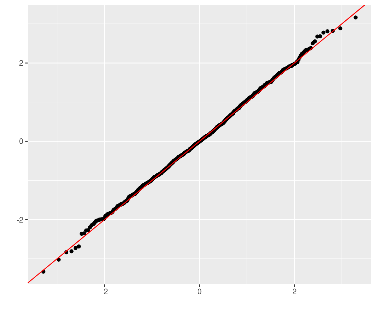
This should be approximately normal, so we Q-Q plot against normality. LGTM.
require(ggplot2)
ph <- qplot(sample = retv[1, , 1], stat = "qq") + geom_abline(intercept = 0,
    slope = 1, colour = "red")
print(ph)
Consider the case of an 8-vector drawn from some population. One
observes some fixed number of independent observations of the vector,
computes the sample covariance matrix, then computes its trace. Using a
madness object, one can automagically estimate the standard
error via the delta method. The sample calculation looks as follows:
genrows <- function(nsim, mu, haSg) {
    p <- length(mu)
    X <- matrix(rnorm(nsim * p), nrow = nsim, ncol = p) %*%
        haSg
    X <- t(rep(mu, nsim) + t(X))
}

p <- 8
set.seed(8644)
true.mu <- array(rnorm(p), dim = c(p, 1))
true.Sigma <- diag(runif(p, min = 1, max = 20))
true.trace <- matrix.trace(true.Sigma)
haSigma <- chol(true.Sigma)

ndays <- 1250

X <- genrows(ndays, true.mu, haSigma)
twom <- twomoments(X)
matt <- matrix.trace(twom$Sigma)

# Now perform some simulations to see if these are
# accurate:

nsim <- 1000
set.seed(23401)
retv <- replicate(nsim, {
    X <- genrows(ndays, true.mu, haSigma)
    twom <- twomoments(X, df = 1)
    matt <- matrix.trace(twom$Sigma)
    marginal.wald <- (val(matt) - true.trace)/sqrt(diag(vcov(matt)))
})
require(ggplot2)
ph <- qplot(sample = as.numeric(retv), stat = "qq") +
    geom_abline(intercept = 0, slope = 1, colour = "red")
print(ph)
Consider the case of a 10-vector drawn from a population with
covariance matrix whose largest eigenvalue is, say, 17.
One observes some fixed number of independent observations of the
10-vector, and computes the sample covariance matrix, then computes the
maximum eigenvalue. Using a madness object, one can
automagically estimate the standard error via the delta method. The
sample calculation looks as follows:
genrows <- function(nsim, mu, haSg) {
    p <- length(mu)
    X <- matrix(rnorm(nsim * p), nrow = nsim, ncol = p) %*%
        haSg
    X <- t(rep(mu, nsim) + t(X))
}

p <- 10
set.seed(123950)
true.mu <- array(rnorm(p), dim = c(p, 1))
true.maxe <- 17
true.Sigma <- diag(c(true.maxe, runif(p - 1, min = 1,
    max = 16)))
haSigma <- chol(true.Sigma)

ndays <- 1250

X <- genrows(ndays, true.mu, haSigma)
twom <- twomoments(X, df = 1)
maxe <- maxeig(twom$Sigma)
print(maxe)
## class: madness
## d maxeig(Sigma)
## calc: -----------------
## d X
## val: 18 ...
## dvdx: 0 1.6 0.0068 -0.16 0.05 -0.0065 0.051 -0.0024 0.032 -0.035 -0.049 0.99 0.0086 -0.2 0.063 -0.0081 0.064 -0.003 0.04 -0.044 -0.062 1.9e-05 -0.00087 0.00028 -3.5e-05 0.00028 -1.3e-05 0.00018 -0.00019 -0.00027 0.01 -0.0064 0.00082 -0.0065 0.00031 -0.0041 0.0045 0.0063 0.001 -0.00026 0.0021 -9.6e-05 0.0013 -0.0014 -0.002 1.7e-05 -0.00026 1.2e-05 -0.00017 0.00018 0.00025 0.001 -9.8e-05 0.0013 -0.0014 -0.002 2.3e-06 -6.1e-05 6.7e-05 9.4e-05 0.00041 -9e-04 -0.0013 0.00049 0.0014 0.00097 ...
## varx: 2.4e-34 9.4e-21 4.2e-20 1.8e-20 1.5e-20 -1.1e-20 -1.1e-20 2.6e-20 -7.5e-21 -4.2e-20 -1.6e-20 2e-19 -6e-20 -3e-20 -2e-20 2.3e-20 2.1e-20 -3.9e-20 1.6e-20 6.4e-20 1.5e-20 5.8e-20 -2.5e-20 -4.4e-20 6.4e-20 5.4e-20 -8.8e-20 3.2e-20 1.4e-19 3.5e-20 1.3e-19 -8.1e-21 2.3e-20 6.6e-21 -1.7e-20 1.5e-20 3.8e-20 6.7e-21 1.6e-19 2.3e-20 1.9e-20 -2.8e-20 7.3e-21 5.9e-20 1e-20 6e-21 -2.1e-20 4.3e-20 -1.5e-20 -7.6e-20 -2.3e-20 1.4e-19 2.6e-20 -1.1e-20 -5e-20 -1.7e-20 4.3e-20 1.8e-20 1e-19 2.8e-20 8.9e-20 -3.9e-20 -1.1e-20 -4.4e-20 -4.4e-20 1.4e-20 ...print(vcov(maxe))## [,1]
## [1,] 0.53Now perform some simulations to see if these are accurate:
nsim <- 1000
set.seed(23401)
retv <- replicate(nsim, {
    X <- genrows(ndays, true.mu, haSigma)
    twom <- twomoments(X, df = 1)
    maxe <- maxeig(twom$Sigma)
    marginal.wald <- (val(maxe) - true.maxe)/sqrt(diag(vcov(maxe)))
})
require(ggplot2)
ph <- qplot(sample = as.numeric(retv), stat = "qq") +
    geom_abline(intercept = 0, slope = 1, colour = "red")
print(ph)
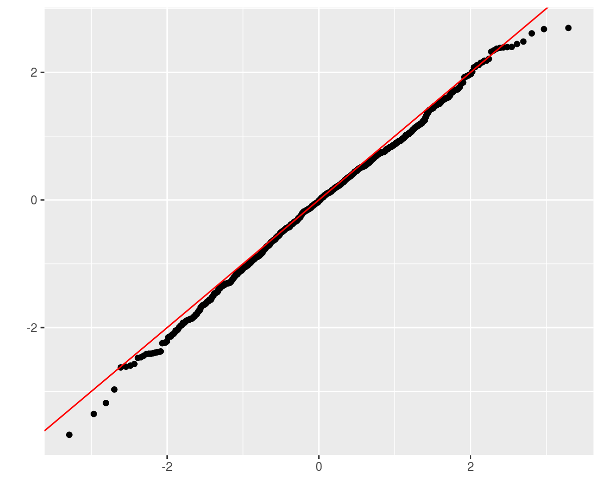
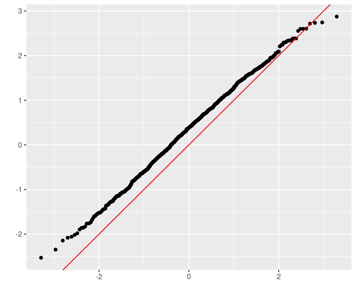
Why the bias? There are a number of possibilities:
An example is in order. Consider the tasting data compiled by Nessie on 86 Scotch whiskies. The data are availble online and look like so:
library(curl)
wsky <- read.csv(curl("https://www.mathstat.strath.ac.uk/outreach/nessie/datasets/whiskies.txt"),
    stringsAsFactors = FALSE)
kable(head(wsky))| RowID | Distillery | Body | Sweetness | Smoky | Medicinal | Tobacco | Honey | Spicy | Winey | Nutty | Malty | Fruity | Floral | Postcode | Latitude | Longitude |
|---|---|---|---|---|---|---|---|---|---|---|---|---|---|---|---|---|
| 1 | Aberfeldy | 2 | 2 | 2 | 0 | 0 | 2 | 1 | 2 | 2 | 2 | 2 | 2 | PH15 2EB | 286580 | 749680 |
| 2 | Aberlour | 3 | 3 | 1 | 0 | 0 | 4 | 3 | 2 | 2 | 3 | 3 | 2 | AB38 9PJ | 326340 | 842570 |
| 3 | AnCnoc | 1 | 3 | 2 | 0 | 0 | 2 | 0 | 0 | 2 | 2 | 3 | 2 | AB5 5LI | 352960 | 839320 |
| 4 | Ardbeg | 4 | 1 | 4 | 4 | 0 | 0 | 2 | 0 | 1 | 2 | 1 | 0 | PA42 7EB | 141560 | 646220 |
| 5 | Ardmore | 2 | 2 | 2 | 0 | 0 | 1 | 1 | 1 | 2 | 3 | 1 | 1 | AB54 4NH | 355350 | 829140 |
| 6 | ArranIsleOf | 2 | 3 | 1 | 1 | 0 | 1 | 1 | 1 | 0 | 1 | 1 | 2 | KA27 8HJ | 194050 | 649950 |
A bizarre question one could ask of this data are whether the taste characteristics are related to the geographic coordinates of the distilleries? One way to pose this is to perform a linear regression of the taste values on the geographic coordinates. This is a many-to-many regression. The Multivariate General Linear Hypothesis is a general hypothesis about the regression coefficients in this case. The ‘usual’ application is the omnibus test of whether all regression coefficients are zero. The MGLH is classically approached by four different tests, which typically give the same answer.
First, we grab the geographic and taste data, prepend a one to the vector, take an outer product and compute the mean and covariance. The MGLH statistics can be posed in terms of the eigenvalues of a certain matrix. Here these are statistics are computed so as to equal zero under the null hypothesis of all zero linear regression coefficient from geography to taste. We get the approximate standard errors from the delta method, and compute Wald statistics.
x <- cbind(1, 1e-05 * wsky[, c("Latitude", "Longitude")])
y <- wsky[, c("Body", "Sweetness", "Smoky", "Medicinal",
    "Tobacco", "Honey", "Spicy", "Winey", "Nutty",
    "Malty", "Fruity", "Floral")]
xy <- cbind(x, y)
# estimate second moment matrix:
xytheta <- theta(xy)
nfeat <- ncol(x)
ntgt <- ncol(y)
GammaB <- xytheta[1:nfeat, nfeat + (1:ntgt)]
SiB <- -solve(xytheta)[nfeat + (1:ntgt), 1:nfeat]
EH <- SiB %*% GammaB
oEH <- diag(ntgt) + EH

HLT <- matrix.trace(oEH) - ntgt
PBT <- ntgt - matrix.trace(solve(oEH))
# this is not the LRT, but log of 1/LRT. sue me.
LRT <- log(det(oEH))
RLR <- maxeig(oEH) - 1
MGLH <- c(HLT, PBT, LRT, RLR)
walds <- val(MGLH)/sqrt(diag(vcov(MGLH)))

# put them together to show them:
preso <- data.frame(type = c("HLT", "PBT", "LRT", "RLR"),
    stat = as.numeric(MGLH), Wald.stat = as.numeric(walds))
kable(preso)| type | stat | Wald.stat |
|---|---|---|
| HLT | 66.6 | 5.0 |
| PBT | 1.7 | 15.6 |
| LRT | 5.2 | 16.8 |
| RLR | 76.0 | 4.8 |
These all cast doubt on the hypothesis of ‘no connection between geography and taste’, although I am accustomed to seeing Wald statistics being nearly equivalent. This is still beta code. We also have the estimated standard error covariance of the vector of MGLH statistics, turned into a correlation matrix here. The four test methods have positively correlated standard errors, meaning we should not be more confident if all four suggest rejecting the null.
print(cov2cor(vcov(MGLH)))## [,1] [,2] [,3] [,4]
## [1,] 1.00 0.15 0.75 0.98
## [2,] 0.15 1.00 0.75 0.11
## [3,] 0.75 0.75 1.00 0.71
## [4,] 0.98 0.11 0.71 1.00The following are cribbed from the unit tests (of which there are never enough). First we define the function which computes approximate derivatives numerically, then test it on some functions:
require(madness)
require(testthat)

apx_deriv <- function(xval, thefun, eps = 1e-09, type = c("forward",
    "central")) {
    type <- match.arg(type)
    yval <- thefun(xval)
    dapx <- matrix(0, length(yval), length(xval))
    for (iii in seq_len(length(xval))) {
        xalt <- xval
        xalt[iii] <- xalt[iii] + eps
        yplus <- thefun(xalt)
        dydx <- switch(type, forward = {
            (yplus - yval)/eps
        }, central = {
            xalt <- xval
            xalt[iii] <- xalt[iii] - eps
            yneg <- thefun(xalt)
            (yplus - yneg)/(2 * eps)
        })
        dapx[, iii] <- as.numeric(dydx)
    }
    dapx
}

test_harness <- function(xval, thefun, scalfun = thefun,
    eps = 1e-07) {
    xobj <- madness(val = xval, vtag = "x", xtag = "x")
    yobj <- thefun(xobj)
    xval <- val(xobj)
    dapx <- apx_deriv(xval, scalfun, eps = eps, type = "central")
    # compute error:
    dcmp <- dvdx(yobj)
    dim(dcmp) <- dim(dapx)

    merror <- abs(dapx - dcmp)
    rerror <- merror/(0.5 * pmax(sqrt(eps), (abs(dapx) +
        abs(dcmp))))
    rerror[dapx == 0 & dcmp == 0] <- 0
    max(abs(rerror))
}

# now test a bunch:
set.seed(2015)

xval <- matrix(1 + runif(4 * 4), nrow = 4)
yval <- matrix(1 + runif(length(xval)), nrow = nrow(xval))
expect_lt(test_harness(xval, function(x) {
    x + x
}), 1e-06)
expect_lt(test_harness(xval, function(x) {
    x * yval
}), 1e-06)
expect_lt(test_harness(xval, function(x) {
    yval/x
}), 1e-06)
expect_lt(test_harness(xval, function(x) {
    x^x
}), 1e-06)
expect_lt(test_harness(xval, function(x) {
    x %*% x
}), 1e-06)
expect_lt(test_harness(xval, function(x) {
    x %*% yval
}), 1e-06)

expect_lt(test_harness(abs(xval), function(x) {
    log(x)
}), 1e-06)
expect_lt(test_harness(xval, function(x) {
    exp(x)
}), 1e-06)
expect_lt(test_harness(abs(xval), function(x) {
    log10(x)
}), 1e-06)
expect_lt(test_harness(xval, function(x) {
    sqrt(x)
}), 1e-06)

expect_lt(test_harness(xval, function(x) {
    matrix.trace(x)
}, function(matx) {
    sum(diag(matx))
}), 1e-06)
expect_lt(test_harness(xval, function(x) {
    colSums(x)
}), 1e-06)
expect_lt(test_harness(xval, function(x) {
    colMeans(x)
}), 1e-06)

expect_lt(test_harness(xval, function(x) {
    vec(x)
}, function(x) {
    dim(x) <- c(length(x), 1)
    x
}), 1e-06)
expect_lt(test_harness(xval, function(x) {
    vech(x)
}, function(x) {
    x <- x[row(x) >= col(x)]
    dim(x) <- c(length(x), 1)
    x
}), 1e-06)

expect_lt(test_harness(xval, function(x) {
    tril(x)
}, function(x) {
    x[row(x) < col(x)] <- 0
    x
}), 1e-06)
expect_lt(test_harness(xval, function(x) {
    triu(x)
}, function(x) {
    x[row(x) > col(x)] <- 0
    x
}), 1e-06)

expect_lt(test_harness(xval, function(x) {
    det(x)
}), 1e-06)
expect_lt(test_harness(xval, function(x) {
    determinant(x, logarithm = TRUE)$modulus
}), 1e-06)
expect_lt(test_harness(xval, function(x) {
    determinant(x, logarithm = FALSE)$modulus
}), 1e-06)

expect_lt(test_harness(xval, function(x) {
    colSums(x)
}), 1e-06)
expect_lt(test_harness(xval, function(x) {
    colMeans(x)
}), 1e-06)
expect_lt(test_harness(xval, function(x) {
    rowSums(x)
}), 1e-06)
expect_lt(test_harness(xval, function(x) {
    rowMeans(x)
}), 1e-06)

set.seed(2015)
zval <- matrix(0.01 + runif(4 * 100, min = 0, max = 0.05),
    nrow = 4)
xval <- tcrossprod(zval)

expect_lt(test_harness(xval, function(x) {
    norm(x, "O")
}), 1e-06)
expect_lt(test_harness(xval, function(x) {
    norm(x, "I")
}), 1e-06)
# Matrix::norm does not support type '2'
expect_lt(test_harness(xval, function(x) {
    norm(x, "2")
}, function(x) {
    base::norm(x, "2")
}), 1e-06)
expect_lt(test_harness(xval, function(x) {
    norm(x, "M")
}), 1e-06)
expect_lt(test_harness(xval, function(x) {
    norm(x, "F")
}), 1e-06)

expect_lt(test_harness(xval, function(x) {
    sqrtm(x)
}), 1e-06)Some functions implicitly break symmetry, which could cause the differentiation process to fail. For example, the ‘chol’ function is to be applied to a symmetric matrix, but only looks at the upper triangular part, ignoring the lower triangular part. This is demonstrated below. For the moment, the only ‘solution’ is to enforce symmetry of the input. Eventually some native functionality around symmetry may be implemented.
set.seed(2015)
zval <- matrix(0.01 + runif(4 * 100, min = 0, max = 0.05),
    nrow = 4)
xval <- tcrossprod(zval)

fsym <- function(x) {
    0.5 * (x + t(x))
}
# this will fail:
# expect_lt(test_harness(xval,function(x) { chol(x)
# }),1e-6)
expect_gte(test_harness(xval, function(x) {
    chol(x)
}), 1.99)
# this will not:
expect_lt(test_harness(xval, function(x) {
    chol(fsym(x))
}), 1e-06)
The functions twomoments and theta respect
the symmetry of the quantities being estimated.
This code is a proof of concept. The methods used to compute derivatives are not (yet) space-efficient or necessarily numerically stable. User assumes all risk.
Derivatives are stored as a matrix in ‘numerator layout’. That is the independent and dependent variable are vectorized, then the derivative matrix has the same number of columns as elements in the dependent variable. Thus the derivative of a 3 by 2 by 5 y with respect to a 1 by 2 by 2 x is a 30 by 4 matrix.